The MNIST Experiment
Creating an MNIST Digit Classifier as part of FastAI DL Course V4 Chapter 4


Building a digit-detection neural net
Hello and welcome to another of my adventures! Today we will be building a digit detection neural network using the MNIST Digits Data Set. This data set is a freely-available set of handwritten digits (0-9) and will be used to train our neural net.
Using this data set we will ”decompose” a simple neural network, which will allow us to see how it looks from the inside. We will also create our loss function, accuracy metric and see how a network learns, all within this exercise.
Before we Start
Doing this small project was and still is one of my favorite projects I have ever done and I am excited to share it with you!
This project does involve some calculus. If you are like me it has been a while and so it will help to go back and review some concepts, including some calculus (derivatives), Deep Learning parameters and hyperparameters.
Once you know these concepts there are some FastAI, pytorch, python functions that made the concepts easier to practice and implement.
Finally, this exercise is based on (FastAI Course)[course.fast.ai] Lesson 4. You want to click the link if you'd like to review some further details regarding this and other exercises.
Data Structure Review
First things first, we need to know what this data looks like. Let's unpack the data and review it. FastAI already has a way for us to download the full MNIST data set. We will download it, unpack it, and see its contents.
In order to generate our dataset, there are some key questions we need to answer:
- How is the data structured?
- Does it have a validation set?
- How is the data labeled?
# This will download the data and get it ready for the us to review the data set contents
path = untar_data(URLs.MNIST)
Path.BASE_PATH = path
path.ls()
Based on the download, we can see that the data is divided into 2 separate data sets, 'testing' (validation) and 'training' sets. Let’s explore the dataset a little more using the function ls().
(path/'training').ls().sorted(), (path/'testing').ls().sorted()
As we can see from the output, both the testing and training datasets contain folders that represents the digit of the images contained within that folder.
Now lets use Image.open() to render one of the images
# Renderding an image from the training set of the digit number 8
Image.open((path/'training'/'8').ls().sorted()[999])

It looks like a very simple image that contains the digit number in black and white. Based on what we learned so far we are able to answer our key questions, which will help us generate our dataset:
How is the data structured?
We have 2 folders 1 for the training data and one for testing data.
Does it have a validation set?
Yes, the testing data set
How is the data labeled?
Within each of the folders (testing and training) we have child folders that represent the digits and finally within those we have our data
Data Set Definition
Using the answers from the questions above we need to come up with a small script that helps us build our data set.
Here are the criteria for building our script:
- Grab all images from both the training and testing folders
- Traverse each folder structure in order to grab all the digit folders within.
- Grab the images within each digit folder and store them in a way we can label and use them for training and validation.
- Use the folder names to generate our labels for each of the images
Let's look at the following script and see how we can accomplish it.
# This grid will be used for tracking our results from processing the images
training_results = create_grid(len((path/'training').ls().sorted()))

# First lets grab all of our images and store the corresponding paths in
# a list so that we can read them
training_folders = (path/'training').ls().sorted()
training_paths = []

# This tensor will contain the label for each of the images in the data set
train_y = tensor([])

# Index for our grid
index = 0

# We need to loop over the different paths and then grab the paths to
# all of our images sorted so that we can load the image into a
# tensor we can use to pass it to model
for digits in training_folders:

    # Grab the digit label in the path of the folder
    label = re.findall("\d",str(digits))

    # Create a label tensor with equal to the number of images for the digit
    label_tensor = tensor([float(label[0])]*len(digits.ls()))
    train_y = torch.cat((train_y, label_tensor),0)

    # Grab all the paths to our images
    training_paths += digits.ls().sorted()

    # Display our results
    process_row(training_results, index, label[0],len(digits.ls()))
    index+=1

train_y = train_y.type(torch.LongTensor)

# We can check the our array of paths tensor shape should be
# (total number images in all folders)
training_results
Script Results
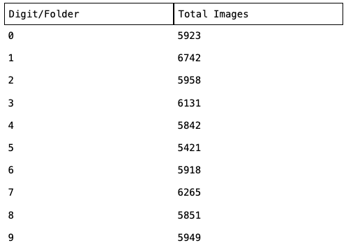
Looks good! The digits and folders appear to be reasonably well distributed.
Now that we have added all of the difits to our training_paths array we can use it to open the images, map the pixel values to a tensor and finally divide them by 255 (max number a pixel value can be) since we want values that fit between 0 and 1 for the resulting images.
# Final we should be able to open the image and store it as a tensor
train_data = torch.stack([tensor(Image.open(o))
                             for o in training_paths.sorted()]).float()/255

# We can check the our tensor shape should be
# (total number images, with a 28 by 28 size) Rank 3 tensor
train_data.shape, train_y.shape
validation_results = create_grid(len((path/'training').ls().sorted()))
validation_labels = (path/'testing').ls().sorted()
validation_paths = []
index = 0
valid_y = tensor([])

for digits in validation_labels:
    label = re.findall("\d",str(digits))
    label_tensor = tensor([float(label[0])]*len(digits.ls()))
    valid_y = torch.cat((valid_y, label_tensor),0)
    validation_paths += digits.ls().sorted()
    process_row(validation_results, index, label[0],len(digits.ls()))
    index+=1

valid_y = valid_y.type(torch.LongTensor)
validation_results
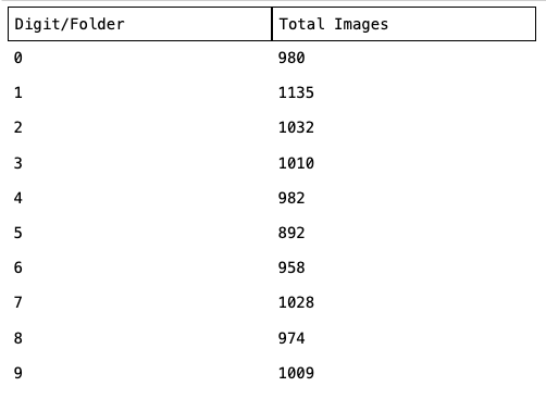
We can now perform the same normalization as in the training set:
- Open the images as a tensor
- Convert the numbers to be between 0 and 1
valid_data = torch.stack([tensor(Image.open(o))
                               for o in validation_paths]).float()/255
valid_data.shape, valid_y.shape
Data Review
When dealing with images something that really helped me was to visualize what was going to happen and experiment a little with the data. Jeremy did something similar in the FastAI course where he opened the image so we could see the underlying data and try to understand and figure out how the machine would process it.
In the next cell we will be grabbing one of the images in the training data, open it with pandas and render the contents using a data frame grid.
a_digit = train_data[51000,:,6:24]
df = pd.DataFrame(a_digit)
df.style.set_properties(**{'font-size':'6pt'}).background_gradient('Greys')
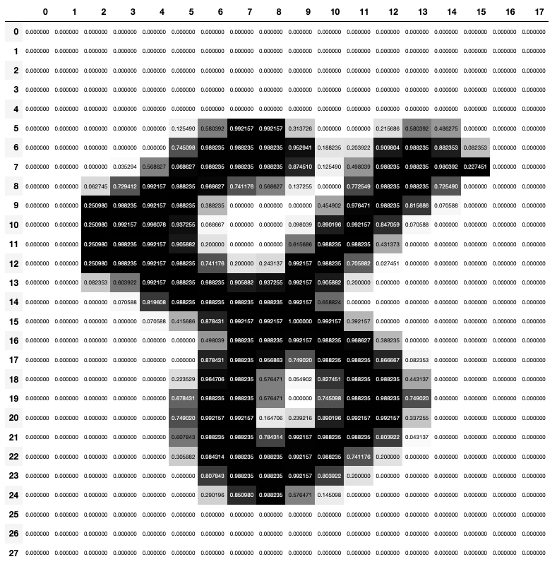
Viewing the data fram grid we can see that each image has 28x28 pixels, and each is represented by a number from 0 to 1 that represents the positive space, but before we are able to use our data sets we need to perform one more transformation.
In order for our neural network to be able to train on our images we need to transform these images into tuples. The main reason for that is that the learner class we will be using accepts a sequence of images with labels, and currently, our images and labels are not paired but stored in separate tensors.
Tuples and Data Sets
We need to transform the training images like the one above into a vector by stacking all the pixels into 1 big column, next create a tuple with the vectorized image and the corresponding label.
Finally, we will create a list of those tuples which will give us our 2 final data sets.
# The 1st value is the index and 2nd will be the image decomposed into a vector
train_x = train_data.view(-1, 28*28)
valid_x = valid_data.view(-1, 28*28)

train_x.shape, valid_x.shape
# This function will create a list of tuples by matching the vector with the corresponding label
# and we can use it in our data loader class and our learner
train_dset = list(zip(train_x,train_y))
valid_dset = list(zip(valid_x,valid_y))
Now the same image above has been transformed into a vector and is followed by the corresponding label at the end of the tuple. (The numbers below represent the image above)
# Grab item 51000 access item 0 in the tuple and
# finally show vector from row 150 to 200
train_dset[51000][0][150:200]
# Grab item 51000 then access item 1 in tuple representing the label
train_dset[51000][1]
Data Set Recap
Let's do a quick recap of everything we have done up to this point. We have:
- Downloaded our images.
- Separated validation and training sets.
- Loaded the images into tensors.
- Transformed the pixel values to values ranging from 0 to 1.
- Transformed them into vectors and pair them with its corresponding labels.
Our data sets are now ready to be used by a model for training and validation. In the next sections we will start loading our data, define our loss and accuracy functions and finally train our model.
Data Loaders
First we need to load the data used for the training and validation, FastAI has a class that will help us pass the training and validation data to our model by generating a mini batch of data.
The Data Loader class can be used even if we are not using a fully developed cnn_learner from FastAI, like, when we are defining our learner manually.
This decoupling of the architecture is extremely cool. It is helpful when people want to build a customized model; we have libraries, classes or pieces of code we can reuse. With the DataLoader class we don't have to reinvent the wheel to create a class or method that help us load our data to our model.
train_dl = DataLoader(train_dset, batch_size=256, shuffle=True)
valid_dl = DataLoader(valid_dset, batch_size=256, shuffle=True)

# The DataLoaders Class is a parent of DataLoader and it holds 2
# DataLoader instances one for training and one for validation
dls = DataLoaders(train_dl, valid_dl)
Measuring model performance: Accuracy and Loss
Accuracy and Loss are 2 representations for model performance that can often be confused because they both reflect performance:
- Accuracy usually represents the average of correct predictions in a model.
- Loss could be thought of as the penalty for making a bad prediction. Loss provides us with a rate of changeto our weights to improve our predictions. Loss takes into account:
- The current learning rate
- Input values
- Parameters for our model
The loss is used in Gradient Descent by the machine to understand with that penalty or “punishment” if the parameters should be updated or not depending on the result of the prediction. The loss function will penalize/punish heavily on worse predictions in proportion to how close the prediction was.
On the other hand accuracy is what helps us, humans, understand the performance of our model so that we can understand and make decisions on whether we should be altering hyperparameters used by the learning process (batch size, number of epochs) to improve the performance of our model.
# This accuracy function will calculate the accuracy comparing the max values of the
# inputs using argmax to get the max values of the passed inputs and then checking it
# aganist the targets and finally calculate the mean

def batch_accuracy(xb, yb):
    xb = np.argmax(xb, 1)
    correct = (xb==yb)
    return correct.float().mean()
def mnist_loss(predictions, targets):
    # When using softmax we need to ensure the number of activations in our
    # last layer matches the number of classes for our model predictions in this case should be 10
    predictions = torch.log_softmax(predictions, 1)
    return F.nll_loss(predictions, targets)
Defining The Neural Network
The definition of a network is not as complex as one might think and you might be surprised (as I was!) that in this case it’s composed of just 3 functions, and how much it can do with only those 3 layers. Here is the definition of a neural net:
simple_net(xb){
  res = xb@w1 + b1
  res = res.max(tensor(0.0))
  res = res@w2 + b2
  return res
}- Layer that performs a matrix multiplication using the values of the image we are trying to predict multiplied by the layer 1 weights then add a bias.
- (Activation) Rectifier linear unity which will basically change any negative result from the previous layer into a 0.
- Final layer which will perform a matrix multiplication with the result of the previous operation multiplied by the weights of layer 2 and add the bias of layer 2.
# Our very simple neural net
simple_net = nn.Sequential(
    nn.Linear(28*28,50),
    nn.ReLU(),
    nn.Linear(50,10)
)
Training the neural net
FastAI has a learner module that enables us to use our own model, optimizer, loss and metrics. The module helps us with:
- Executing the training epochs.
- Calling our optimizer to update our parameters.
- Using the data loaders pass the mini batches to the training.
- Calling our metric functions.
- Give us an output of our training.
Similar to DataLoaders class, this module is very helpful. The learner module decouples the API and supports advanced workflows by enabling users to customize every detail within the model including weight optmization, metrics, and more.
# Lets create our lerner, using our, DataLoaders instance, the simple neural net,
# optimizer, loss and accuracy functions
learn = Learner(dls, simple_net, opt_func=SGD,
                loss_func=mnist_loss, metrics=batch_accuracy)
learn.fit(40, 0.1)
Training Results
As you can see after 40 epochs (previous table only shows the last 20 epochs) of training our new model we have a prediction accuracy of 97% and our training and validation loss less that is less than 10% which is telling us our model is really efficient and accurate when making predictions of handwritten digits.
Visualizing Layer Features
So far we were able to create our data set, define our simple neural net, train and validate it and now lets try to visualize the features its uses to perform and recognize the digits.
We will use the parameters stored in our model and generate a small image representing the features in the network that it recognizes. I loved this part of the exercise since it's where I could "see" how our network defines the features on the layer/s.
The nn.Sequential function used in our model stores the different functions in a list. We can use the index to grab the layer we want to use for the rendering (which is layer 0).
simple_net[0].parameters()You will see that the line above contains a tensor with 50 features, each containing a vector of size 784. We will use what we learned earlier to transform the vector into a 28x28 tensor and finally use the show_images method to render that tensor as an image.
w, b = simple_net[0].parameters()
w.shape
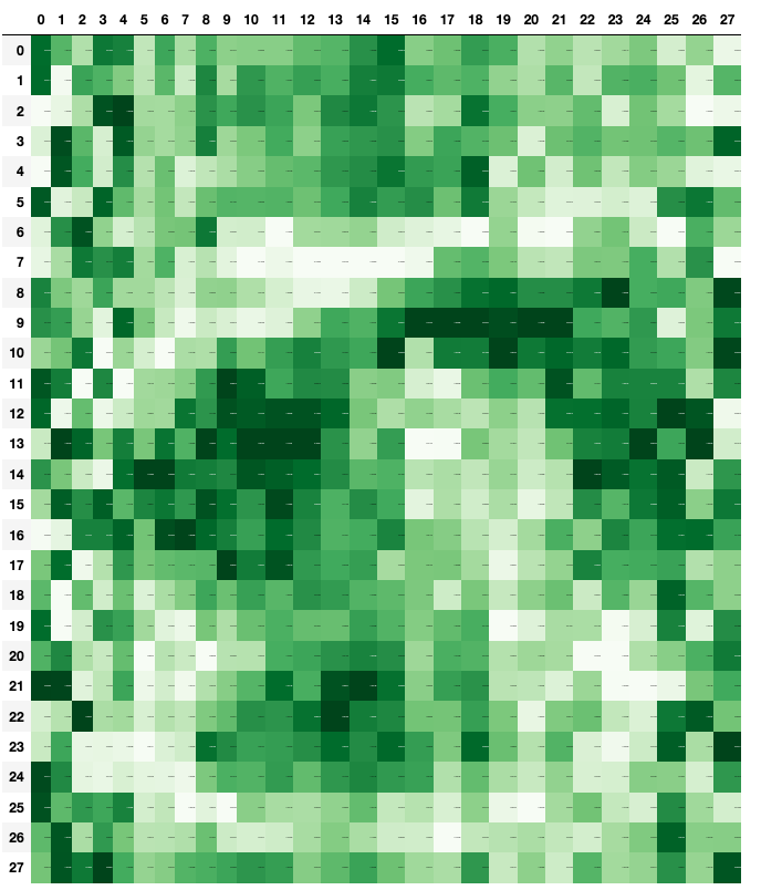
# We can also render a feature using pandas and do it on a grey scale
df2 = pd.DataFrame(w[1].view(28,28)*-1)
df2.style.set_properties(**{'font-size':'1pt'}).background_gradient('Greens')
layer_index = 0
layers_to_render = [0]

# We will use these arrays to store the images and the titles of each of them
images = []
titles = []

# Finally let's loop the layers of the nn.Sequetial
for layer in simple_net:
    if layer_index in layers_to_render:
        index = 0;
        w, b = layer.parameters()

        # Finally we can change the tensor to a 28 by 28 to render the layers
        for feature in w:
            images.append(feature.view(28,28))
            titles.append(str(f'Feature: {index}'))
            index+=1
    layer_index+=1

show_images(images, titles=titles, nrows=8, ncols=5, imsize=4)

Summary
Congratulations making it to the end, I really appreciate you joining me in my journey through Deep Learning journey!
In this exercise we learned about the different modules FastAI exposes and how we can use them to build our custom model:
- DataLoader
- DataLoaders
- Learner
We created our accuracy and loss function and also loaded the data into data loaders that helped us when we were training our model.
We trained a digit detection model with 96using those modules and were able to create an efficient model that recognizes handwritten digits from 0 to 9 with 97% accuracy.
Finally we explored the parameters of the resulting model and a potential path to render the features a model might use, and how they look when visualized.
I hope this was helpful, interesting and fun to build for you as it was for me,
Special thanks to my friend Josh Fleshner for helping me with language and editing of this blog post.
Thanks again and see you on my next adventure.
Resources and References
- Jeremy Howard, Rachel Thomas and Sylvain Gugger, FastAI Course, https://course.fast.ai/videos/?lesson=4
- Grant Sanderson, The Essence of Calculus, 3blue1brown, https://youtube.com/playlist?list=PLZHQObOWTQDMsr9K-rj53DwVRMYO3t5Yr
- Tuples https://docs.python.org/3/tutorial/datastructures.html#tuples-and-sequences
- Jason Brownlee, What is the Difference Between a Parameter and a Hyperparameter?, Machine Learning Mastery, Available from https://machinelearningmastery.com/difference-between-a-parameter-and-a-hyperparameter/